Types, vectors, and functions in R
2020-08-22
1 / 74
Vectors and Types
2 / 74
Vectors
c(1, 3, 5)
c(TRUE, FALSE, TRUE, TRUE)
c("red", "blue")
3 / 74
Vectors
4 / 74
Vectors
Vectors have 1 dimension
5 / 74
Vectors
Vectors have 1 dimension
Vectors have a length.
length(c("blue", "red"))
6 / 74
Vectors
Vectors have 1 dimension
Vectors have a length.
length(c("blue", "red"))
length(c("blue", "red"))Some vectors have names.
names(c("x" = 1, "y = 1))
7 / 74
Vectors
Vectors have 1 dimension
Vectors have a length.
length(c("blue", "red"))
length(c("blue", "red"))Some vectors have names.
names(c("x" = 1, "y = 1))
names(c("x" = 1, "y = 1))Vectors have types
8 / 74
Types
Numeric/double
Integer
Factor
Character
Logical
Dates
9 / 74
Packages to work with types:
Strings/character: stringr
10 / 74
Packages to work with types:
Strings/character: stringr
Factors: forcats
11 / 74
Packages to work with types:
Strings/character: stringr
Factors: forcats
Dates: lubridate
12 / 74
Making vectors
1:3## [1] 1 2 313 / 74
Making vectors
1:3## [1] 1 2 3c(1, 2, 3)## [1] 1 2 313 / 74
Making vectors
1:3## [1] 1 2 3c(1, 2, 3)## [1] 1 2 3rep(1, 3)## [1] 1 1 113 / 74
Making vectors
1:3## [1] 1 2 3c(1, 2, 3)## [1] 1 2 3rep(1, 3)## [1] 1 1 1seq(from = 1, to = 3, by = .5)## [1] 1.0 1.5 2.0 2.5 3.013 / 74
Your Turn 1
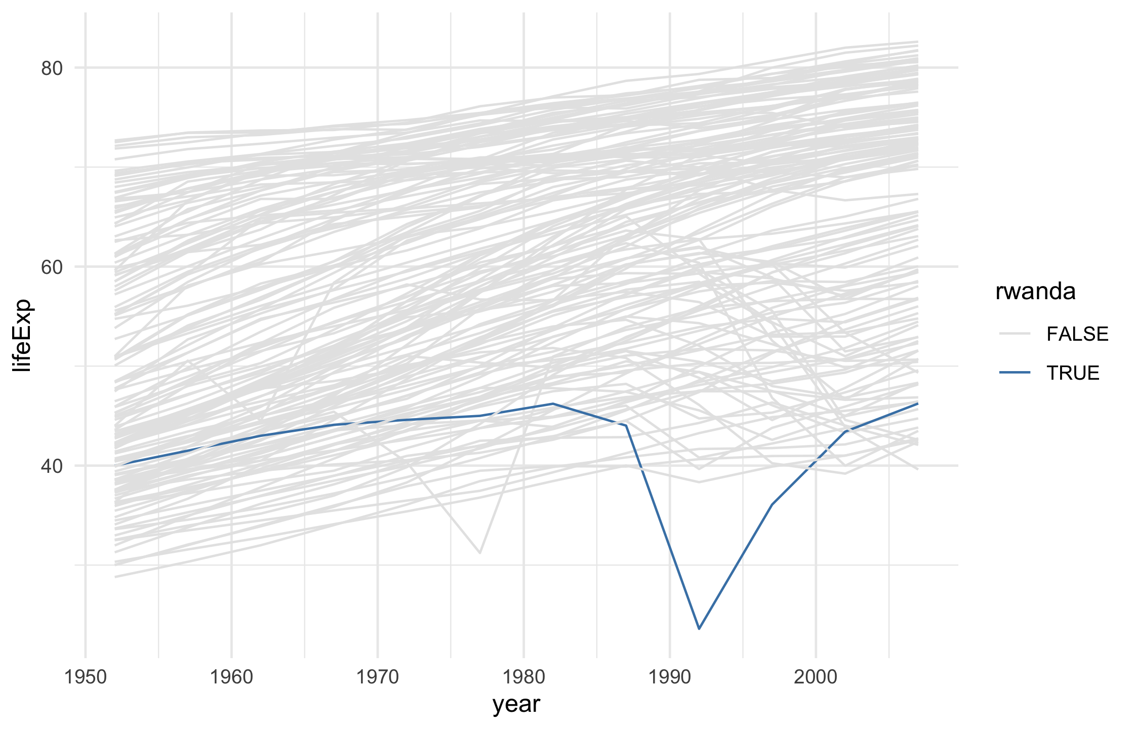
Create a character vector of colors using c(). Use the colors "grey90" and "steelblue". Assign the vector to a name.
Use the vector you just created to change the colors in the plot below using scale_color_manual(). Pass it using the values argument.
14 / 74
Your Turn 1
cols <- c("grey90", "steelblue")gapminder %>% mutate(rwanda = ifelse(country == "Rwanda", TRUE, FALSE)) %>% ggplot(aes(year, lifeExp, color = rwanda, group = country)) + geom_line() + scale_color_manual(values = cols) + theme_minimal()15 / 74
Your Turn 1

16 / 74
Working with vectors
Subset vectors with [] or [[]]
x <- c(1, 5, 7)17 / 74
Working with vectors
Subset vectors with [] or [[]]
x <- c(1, 5, 7)x[2]## [1] 517 / 74
Working with vectors
Subset vectors with [] or [[]]
x <- c(1, 5, 7)x[2]## [1] 5x[[2]]## [1] 517 / 74
Working with vectors
Subset vectors with [] or [[]]
x <- c(1, 5, 7)x[2]## [1] 5x[[2]]## [1] 5x[c(FALSE, TRUE, FALSE)]## [1] 517 / 74
Working with vectors
Modify elements
x## [1] 1 5 718 / 74
Working with vectors
Modify elements
x## [1] 1 5 7x[2] <- 10018 / 74
Working with vectors
Modify elements
x## [1] 1 5 7x[2] <- 100x## [1] 1 100 718 / 74
Modify elements
x## [1] 1 100 719 / 74
Modify elements
x## [1] 1 100 7x[x > 10] <- NA19 / 74
Modify elements
x## [1] 1 100 7x[x > 10] <- NAx## [1] 1 NA 719 / 74
20 / 74
cols <- c("grey90", "steelblue")gapminder %>% mutate(rwanda = ifelse(country == "Rwanda", TRUE, FALSE)) %>% ggplot(aes(year, lifeExp, color = rwanda, group = country)) + geom_line() + scale_color_manual(values = cols) + theme_minimal()21 / 74
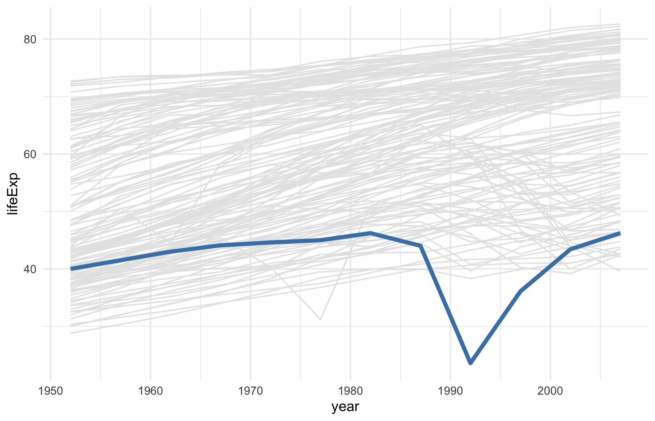
cols <- c("grey90", "steelblue") gapminder %>% mutate(rwanda = ifelse(country == "Rwanda", TRUE, FALSE)) %>% ggplot(aes(year, lifeExp, group = country)) + geom_line( data = function(x) filter(x, !rwanda), color = cols[1] ) + theme_minimal()22 / 74
cols <- c("grey90", "steelblue") gapminder %>% mutate(rwanda = ifelse(country == "Rwanda", TRUE, FALSE)) %>% ggplot(aes(year, lifeExp, color = rwanda, group = country)) + geom_line( data = function(x) filter(x, !rwanda), color = cols[1] ) + geom_line( data = function(x) filter(x, rwanda), color = cols[2], size = 1.5 ) + theme_minimal()23 / 74
24 / 74
Your Turn 2
Create a numeric vector that has the following values: 3, 5, NA, 2, and NA.
Try using sum(). Then add na.rm = TRUE.
Check which values are missing with is.na(); save the results to a new object and take a look
Change all missing values of x to 0
Try sum() again without na.rm = TRUE.
25 / 74
Your Turn 2
x <- c(3, 5, NA, 2, NA)sum(x)## [1] NA26 / 74
Your Turn 2
sum(x, na.rm = TRUE)## [1] 1027 / 74
Your Turn 2
x_missing <- is.na(x)x_missing## [1] FALSE FALSE TRUE FALSE TRUEx[x_missing] <- 0x## [1] 3 5 0 2 0sum(x)## [1] 1028 / 74
Writing Functions
29 / 74
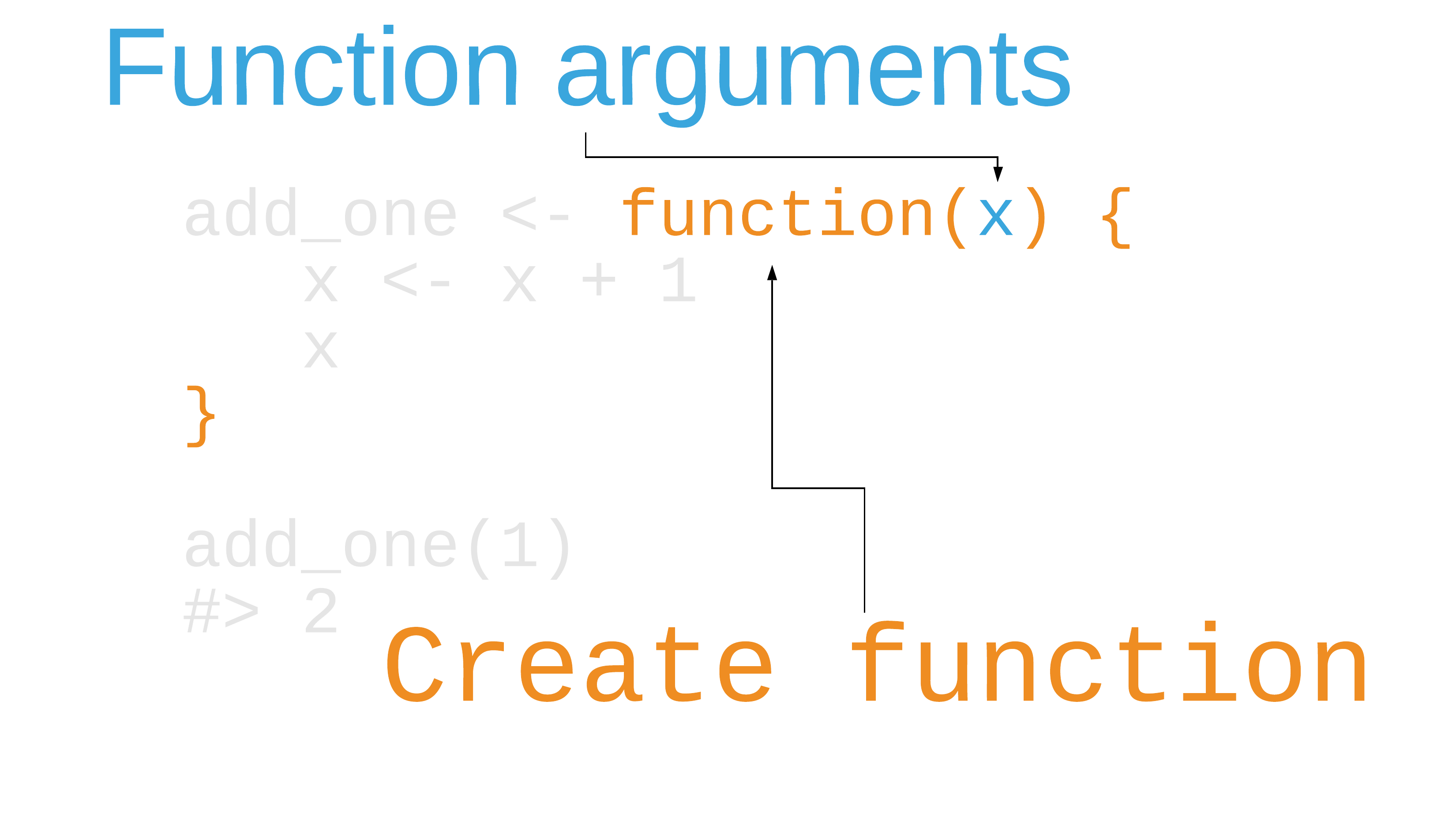
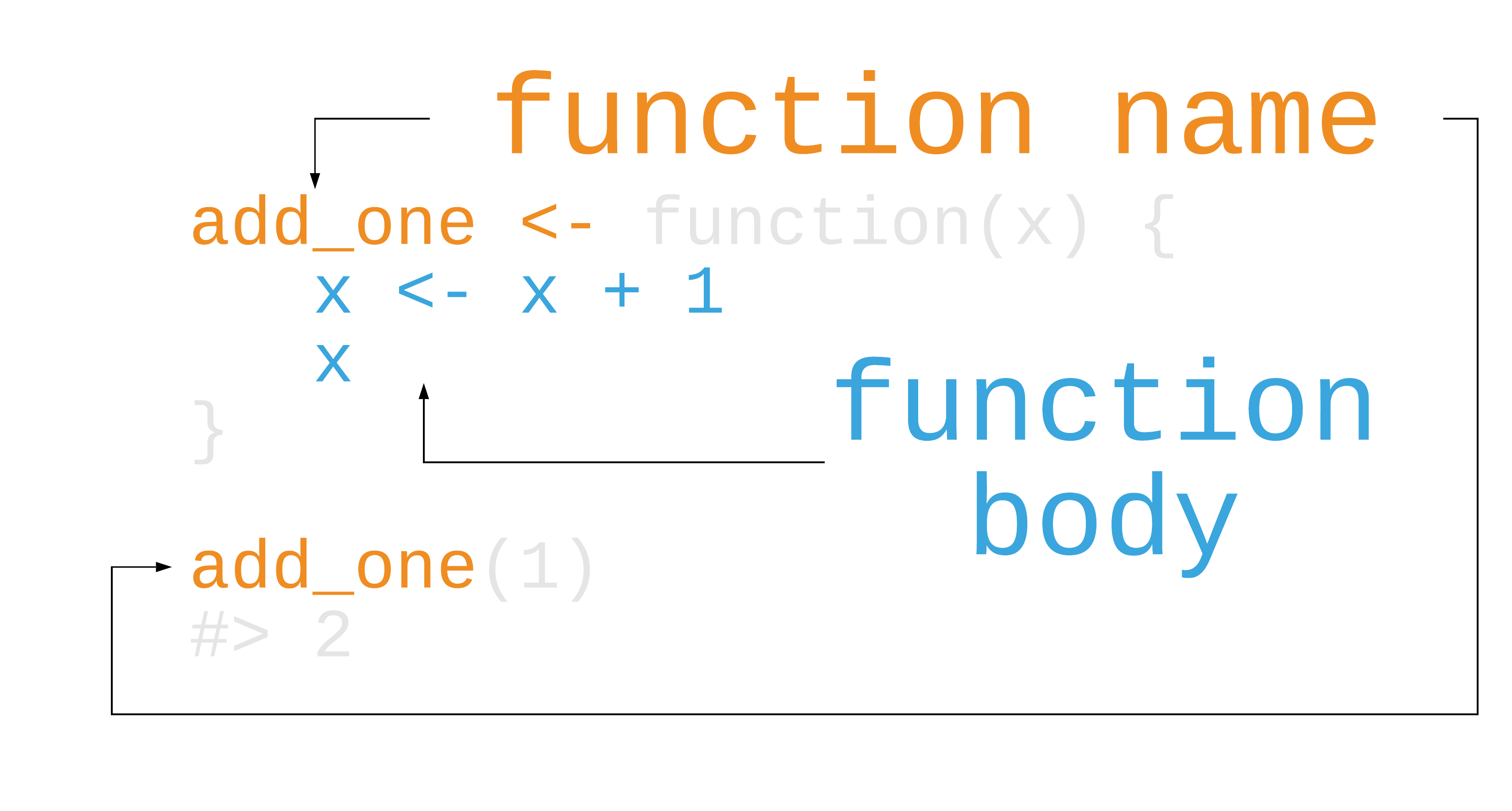
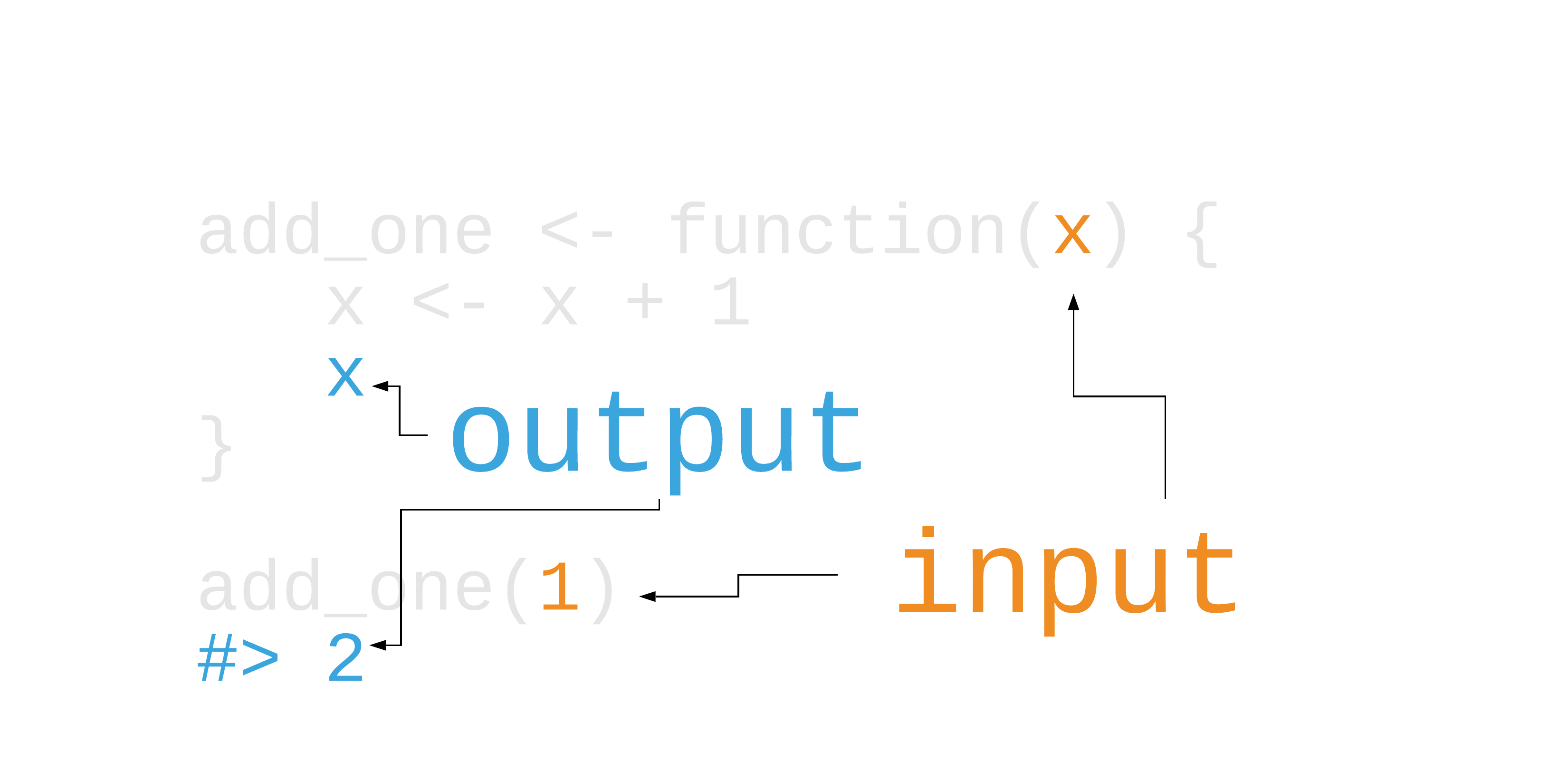
Writing functions

30 / 74
Writing functions
31 / 74
Writing functions
32 / 74
Writing functions
33 / 74
Your Turn 3
Create a function called sim_data that doesn't take any arguments.
In the function body, we'll return a tibble.
For x, have rnorm() return 50 random numbers.
For sex, use rep() to create 50 values of "male" and "female". Hint: You'll have to give rep() a character vector. for the first argument. The times argument is how many times rep() should repeat the first argument, so make sure you 3. account for that.
For age() use the sample() function to sample 50 numbers from 25 to 50 with replacement.
Call sim_data()
34 / 74
Your Turn 3
sim_data <- function() { tibble( x = rnorm(50), sex = rep(c("male", "female"), times = 25), age = sample(25:50, size = 50, replace = TRUE) )}sim_data()35 / 74
Your Turn 3
sim_data <- function() { tibble( x = rnorm(50), sex = rep(c("male", "female"), times = 25), age = sample(25:50, size = 50, replace = TRUE) )}sim_data()36 / 74
Your Turn 3
sim_data <- function() { tibble( x = rnorm(50), sex = rep(c("male", "female"), times = 25), age = sample(25:50, size = 50, replace = TRUE) )}sim_data()37 / 74
Your Turn 3
sim_data <- function() { tibble( x = rnorm(50), sex = rep(c("male", "female"), times = 25), age = sample(25:50, size = 50, replace = TRUE) )}sim_data()38 / 74
Your Turn 3
## # A tibble: 50 x 3## x sex age## <dbl> <chr> <int>## 1 0.312 male 42## 2 -0.387 female 25## 3 -0.0210 male 38## 4 1.38 female 33## 5 0.796 male 30## 6 -0.996 female 29## 7 -0.442 male 38## 8 0.00711 female 28## 9 1.16 male 45## 10 0.116 female 49## # … with 40 more rows39 / 74
E-Values
The strength of unmeasured confounding required to explain away a value
40 / 74
E-Values
The strength of unmeasured confounding required to explain away a value
Rate ratio: 3.9 = E-value: 7.3
41 / 74
Your Turn 4
Write a function to calculate an E-Value given an RR.
Call the function evalue and give it an argument called estimate. In the body of the function, calculate the E-Value using estimate + sqrt(estimate * (estimate - 1))
Call evalue() for a risk ratio of 3.9
42 / 74
Your Turn 4
evalue <- function(estimate) { estimate + sqrt(estimate * (estimate - 1))}43 / 74
Your Turn 4
evalue <- function(estimate) { estimate + sqrt(estimate * (estimate - 1))}evalue(3.9)## [1] 7.26303443 / 74
Control Flow
if (PREDICATE) { true_result}44 / 74
Control Flow
if (PREDICATE) { true_result}if (PREDICATE) { true_result} else { default_result}44 / 74
Control Flow
if (PREDICATE) { true_result}if (PREDICATE) { true_result} else { default_result}if (PREDICATE) { true_result} else if (ANOTHER_PREDICATE) { true_result} else { default_result}44 / 74
Other functions to control flow
ifelse(PREDICATE, true_result, false_result)dplyr::case_when( PREDICATE ~ true_result, PREDICATE ~ true_result, TRUE ~ default_result)switch( x, value1 = result, value2 = result)45 / 74
Validation and stopping
if (is.numeric(x))
stop(), warn()
46 / 74
Validation and stopping
if (is.numeric(x))
stop(), warn()
function(x) { if (is.numeric(x)) stop("x must be a character") # do something with a character}46 / 74
Your Turn 5
Use if () together with is.numeric() to make sure estimate is a number. Remember to use ! for not.
If the estimate is less than 1, set estimate to be equal to 1 / estimate.
Call evalue() for a risk ratio of 3.9. Then try 0.80. Then try a character value.
47 / 74
Your Turn 5
evalue <- function(estimate) { if (!is.numeric(estimate)) stop("`estimate` must be numeric") if (estimate < 1) estimate <- 1 / estimate estimate + sqrt(estimate * (estimate - 1))}48 / 74
Your Turn 5
evalue(3.9)## [1] 7.263034evalue(.80)## [1] 1.809017evalue("3.9")## Error in evalue("3.9"): `estimate` must be numeric49 / 74
Your Turn 6
Add a new argument called type. Set the default value to "rr"
Check if type is equal to "or". If it is, set the value of estimate to be sqrt(estimate)
Call evalue() for a risk ratio of 3.9. Then try it again with type = "or".
50 / 74
Your Turn 6
evalue <- function(estimate, type = "rr") { if (!is.numeric(estimate)) stop("`estimate` must be numeric") if (type == "or") estimate <- sqrt(estimate) if (estimate < 1) estimate <- 1 / estimate estimate + sqrt(estimate * (estimate - 1))}51 / 74
Your Turn 6
evalue(3.9)## [1] 7.263034evalue(3.9, type = "or")## [1] 3.36234252 / 74
Your Turn 7: Challenge!
Create a new function called transform_to_rr with arguments estimate and type.
Use the same code above to check if type == "or" and transform if so. Add another line that checks if type == "hr". If it does, transform the estimate using this formula: (1 - 0.5^sqrt(estimate)) / (1 - 0.5^sqrt(1 / estimate)).
Move the code that checks if estimate < 1 to transform_to_rr (below the OR and HR transformations)
Return estimate
In evalue(), change the default argument of type to be a character vector containing "rr", "or", and "hr".
Get and validate the value of type using match.arg(). Follow the pattern argument_name <- match.arg(argument_name)
Transform estimate using transform_to_rr(). Don't forget to pass it both estimate and type!
53 / 74
Your Turn 7: Challenge!
transform_to_rr <- function(estimate, type) { if (type == "or") estimate <- sqrt(estimate) if (type == "hr") { estimate <- (1 - 0.5^sqrt(estimate)) / (1 - 0.5^sqrt(1 / estimate)) } if (estimate < 1) estimate <- 1 / estimate estimate}evalue <- function(estimate, type = c("rr", "or", "hr")) { # validate arguments if (!is.numeric(estimate)) stop("`estimate` must be numeric") type <- match.arg(type) # calculate evalue estimate <- transform_to_rr(estimate, type) estimate + sqrt(estimate * (estimate - 1))}54 / 74
Your Turn 7: Challenge!
transform_to_rr <- function(estimate, type) { if (type == "or") estimate <- sqrt(estimate) if (type == "hr") { estimate <- (1 - 0.5^sqrt(estimate)) / (1 - 0.5^sqrt(1 / estimate)) } if (estimate < 1) estimate <- 1 / estimate estimate}evalue <- function(estimate, type = c("rr", "or", "hr")) { # validate arguments if (!is.numeric(estimate)) stop("`estimate` must be numeric") type <- match.arg(type) # calculate evalue estimate <- transform_to_rr(estimate, type) estimate + sqrt(estimate * (estimate - 1))}55 / 74
Your Turn 7: Challenge!
transform_to_rr <- function(estimate, type) { if (type == "or") estimate <- sqrt(estimate) if (type == "hr") { estimate <- (1 - 0.5^sqrt(estimate)) / (1 - 0.5^sqrt(1 / estimate)) } if (estimate < 1) estimate <- 1 / estimate estimate}evalue <- function(estimate, type = c("rr", "or", "hr")) { # validate arguments if (!is.numeric(estimate)) stop("`estimate` must be numeric") type <- match.arg(type) # calculate evalue estimate <- transform_to_rr(estimate, type) estimate + sqrt(estimate * (estimate - 1))}56 / 74
Your Turn 7: Challenge!
evalue(3.9)## [1] 7.263034evalue(3.9, type = "or")## [1] 3.362342evalue(3.9, type = "hr")## [1] 4.474815evalue(3.9, type = "rd")## Error in match.arg(type): 'arg' should be one of "rr", "or", "hr"57 / 74
Pass the dots: ...
58 / 74
Pass the dots: ...
select_gapminder <- function(...) { gapminder %>% select(...)}select_gapminder(pop, year)58 / 74
Pass the dots: ...
select_gapminder <- function(...) { gapminder %>% select(...)}select_gapminder(pop, year)59 / 74
Pass the dots: ...
## # A tibble: 1,704 x 2## pop year## <int> <int>## 1 8425333 1952## 2 9240934 1957## 3 10267083 1962## 4 11537966 1967## 5 13079460 1972## 6 14880372 1977## 7 12881816 1982## 8 13867957 1987## 9 16317921 1992## 10 22227415 1997## # … with 1,694 more rows60 / 74
Your Turn 8
Use ... to pass the arguments of your function, filter_summarize(), to filter().
In summarize, get the n and mean life expectancy for the data set
Check filter_summarize() with year == 1952.
Try filter_summarize() again for 2002, but also filter countries that have "and" in the country name. Use str_detect() from the stringr package.
61 / 74
Your Turn 8
filter_summarize <- function(...) { gapminder %>% filter(...) %>% summarize(n = n(), mean_lifeExp = mean(lifeExp))}62 / 74
filter_summarize(year == 1952)## # A tibble: 1 x 2## n mean_lifeExp## <int> <dbl>## 1 142 49.1filter_summarize(year == 2002, str_detect(country, " and "))## # A tibble: 1 x 2## n mean_lifeExp## <int> <dbl>## 1 4 69.963 / 74
Programming with dplyr, ggplot2, and friends
plot_hist <- function(x) { ggplot(gapminder, aes(x = x)) + geom_histogram()}64 / 74
Programming with dplyr, ggplot2, and friends
plot_hist <- function(x) { ggplot(gapminder, aes(x = x)) + geom_histogram()}plot_hist(lifeExp)## Error in FUN(X[[i]], ...): object 'lifeExp' not found
65 / 74
Programming with dplyr, ggplot2, and friends
plot_hist <- function(x) { ggplot(gapminder, aes(x = x)) + geom_histogram()}plot_hist("lifeExp")## Error: StatBin requires a continuous x variable: the x variable is discrete.Perhaps you want stat="count"?
66 / 74
Curly-curly
plot_hist <- function(x) { ggplot(gapminder, aes(x = {{x}})) + geom_histogram()}67 / 74
Curly-curly
plot_hist <- function(x) { ggplot(gapminder, aes(x = {{x}})) + geom_histogram()}plot_hist(lifeExp)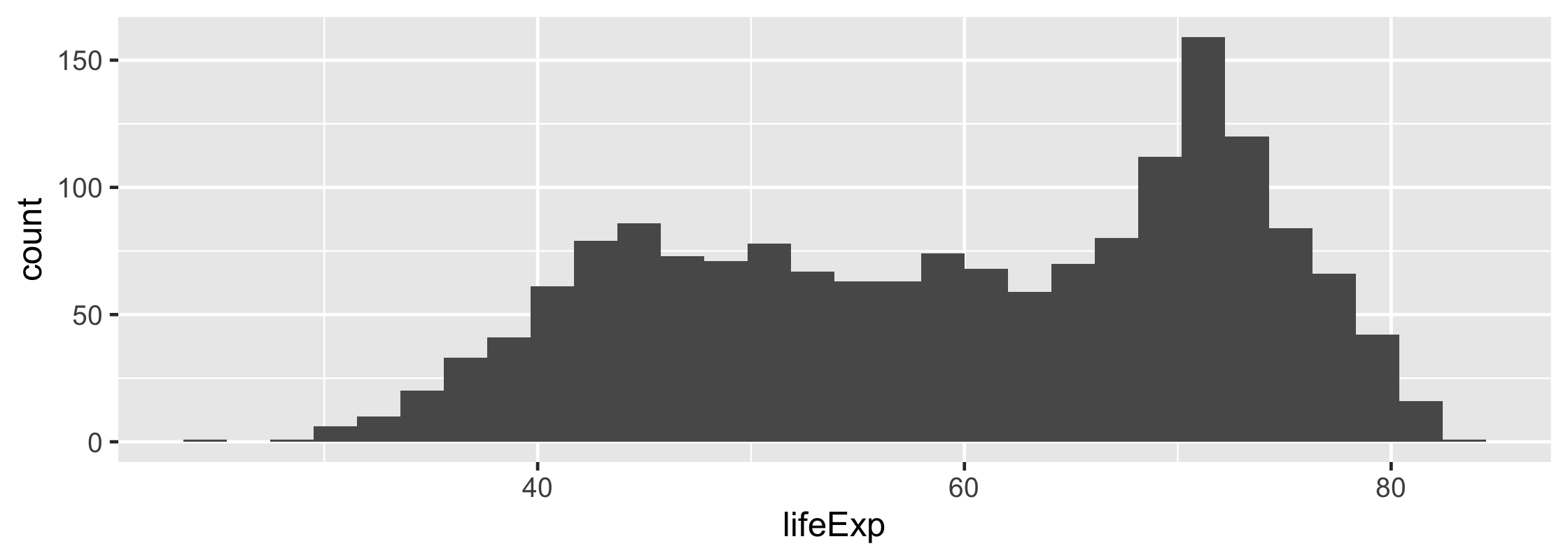
68 / 74
Your turn 9
Filter gapminder by year using the value of .year (notice the period before hand!). You do NOT need curly-curly for this. (Why is that?)
Arrange it by the variable. Don't forget to wrap it in curly-curly!
Make a scatter plot. Use variable for x. For y, we'll use country, but to keep it in the order we arranged it by, we'll turn it into a factor. Wrap the the factor() call with fct_inorder(). Check the help page if you want to know more about what this is doing.
69 / 74
Your turn 9
top_barplot <- function(variable, .year) { gapminder %>% filter(year == .year) %>% arrange(desc({{variable}})) %>% # take the 10 lowest values tail(10) %>% ggplot(aes(x = {{variable}}, y = fct_inorder(factor(country)))) + geom_point() + theme_minimal()}70 / 74
Your turn 9
top_barplot <- function(variable, .year) { gapminder %>% filter(year == .year) %>% arrange(desc({{variable}})) %>% # take the 10 lowest values tail(10) %>% ggplot(aes(x = {{variable}}, y = fct_inorder(factor(country)))) + geom_point() + theme_minimal()}71 / 74
Your turn 9
top_barplot(lifeExp, 2002)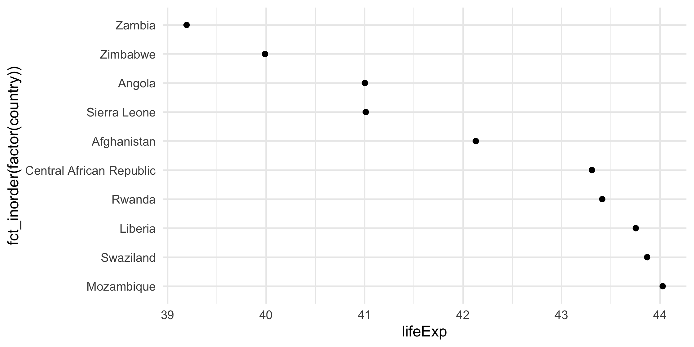
72 / 74
Your turn 9
top_barplot(lifeExp, 2002) + labs(x = "Life Expectancy", y = "Country")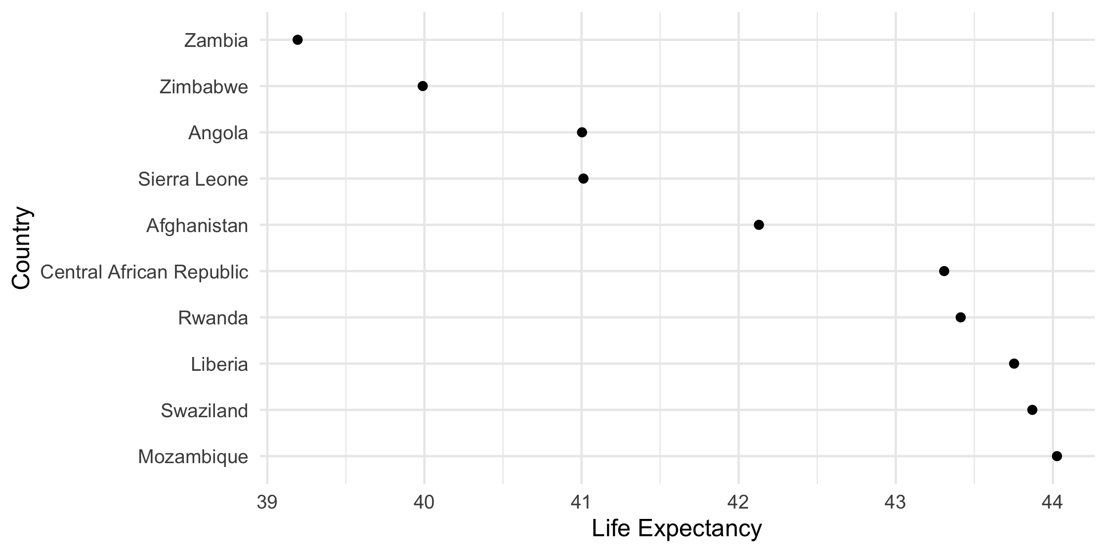
73 / 74
Resources
R for Data Science: A comprehensive but friendly introduction to the tidyverse. Free online.
Advanced R, 2nd ed.: Detailed guide to how R works and how to make your code better. Free online.
RStudio Primers: Free interactive courses in the Tidyverse
74 / 74