Dynamic documents in R
reproducible research with R Markdown
2020-08-22
1 / 51
Artwork by @allison_horst
2 / 51
R Markdown
3 / 51
R Markdown
Authoring framework: code and text in same document
3 / 51
R Markdown
Authoring framework: code and text in same document
Reproducible: re-run your analysis
3 / 51
R Markdown
Authoring framework: code and text in same document
Reproducible: re-run your analysis
Flexible: Output to different formats easily
3 / 51
knitting
4 / 51
Your turn 1
Create a new R Markdown file. Go to File > New File > R Markdown. Press OK. Save the file and press the "Knit" button above.
5 / 51
6 / 51
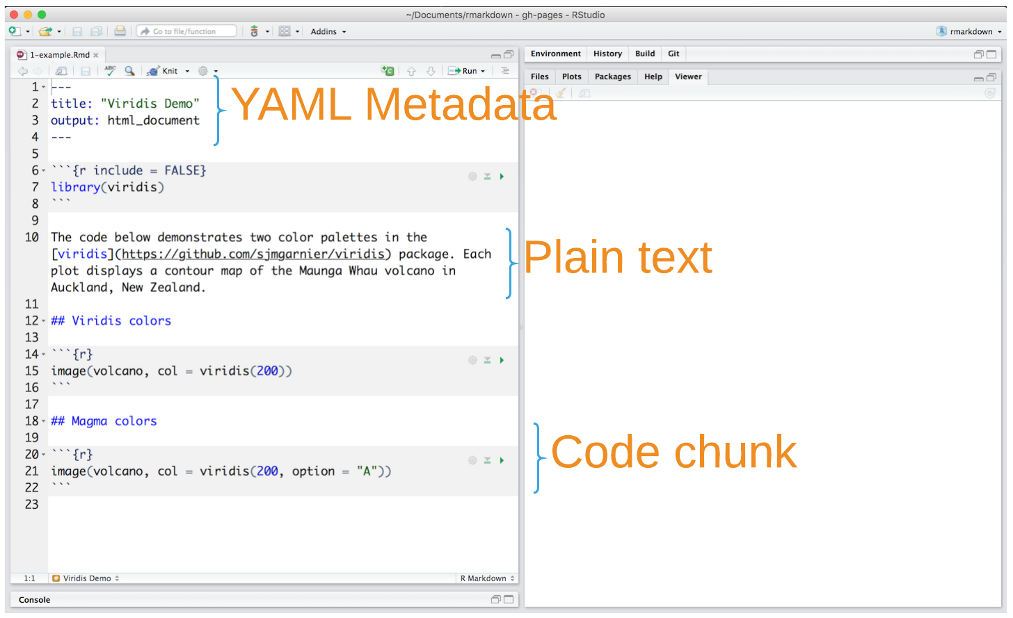
R Markdown
Prose
Code
Metadata
7 / 51
R Markdown
Prose = Markdown
Code
Metadata
8 / 51
Basic Markdown Syntax
*italic* **bold**_italic_ __bold__9 / 51
Basic Markdown Syntax
# Header 1## Header 2### Header 310 / 51
Basic Markdown Syntax
* Item 1* Item 2 + Item 2a + Item 2b1. Item 12. Item 211 / 51
Basic Markdown Syntax
http://example.com[linked phrase](http://example.com)12 / 51
Basic Markdown Syntax
13 / 51
Basic Markdown Syntax
$equation$$$ equation $$14 / 51
Basic Markdown Syntax
superscript^2^~~strikethrough~~15 / 51
Your turn 2
Do the ten-twenty minute tutorial on markdown at https://commonmark.org/help/tutorial. Let us know if you need help!
16 / 51
Your turn 3
Use Markdown syntax to stylize the text from the Gapminder website below. Experiment with bolding, italicizing, making lists, etc.
17 / 51
R Markdown
Prose
Code = R code chunks
Metadata
18 / 51
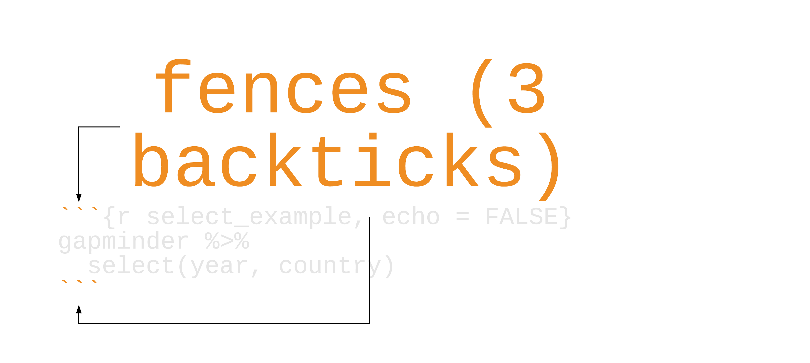
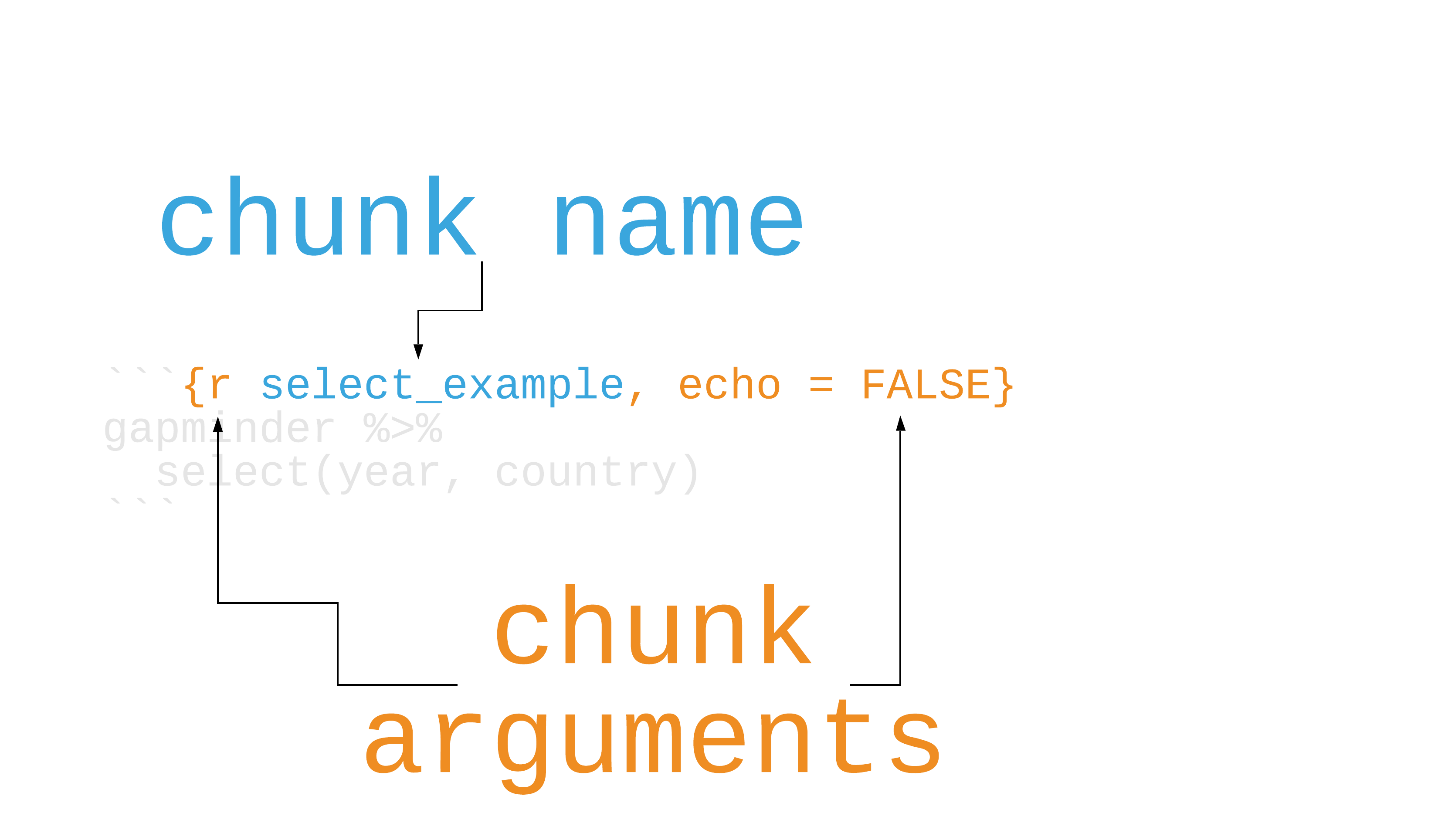
Code chunks

19 / 51
Code chunks
20 / 51
Code chunks
21 / 51
Chunk options
| Option | Effect |
|---|---|
include = FALSE |
run the code but don't print it or results |
eval = FALSE |
don't evaluate the code |
echo = FALSE |
run the code and output but don't print code |
message = FALSE |
don't print messages (e.g. from a function) |
warning = FALSE |
don't print warnings |
fig.cap = "Figure 1 |
caption output plot with "Figure 1" |
22 / 51
Chunk options
| Option | Effect |
|---|---|
include = FALSE |
run the code but don't print it or results |
eval = FALSE |
don't evaluate the code |
echo = FALSE |
run the code and output but don't print code |
message = FALSE |
don't print messages (e.g. from a function) |
warning = FALSE |
don't print warnings |
fig.cap = "Figure 1 |
caption output plot with "Figure 1" |
See the knitr web page
22 / 51
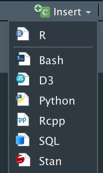
Engines
52! Including Python, Julia, C++, SQL, SAS, and Stata
23 / 51
Insert code chunks with cmd/ctrl + alt/option + I
24 / 51
Edit code chunk options
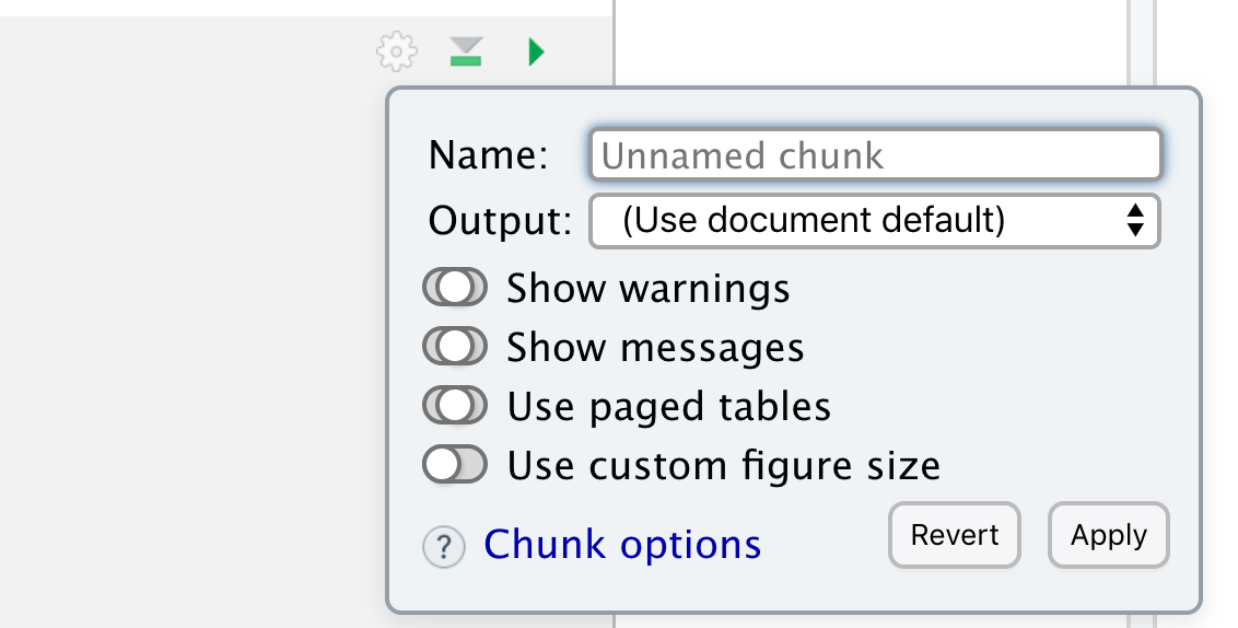
25 / 51
Your turn 4 (open exercises.Rmd)
Create a code chunk. You can type it in manually, use the keyboard short-cut (Cmd/Ctrl + Option/Alt + I), or use the "Insert" button above. Put the following code in it:
gapminder %>% slice(1:5) %>% knitr::kable()Knit the document
26 / 51
Your turn 5
Add echo = FALSE to the code chunk above and re-knit
Remove echo = FALSE from the code chunk and move it to knitr::opts_chunk$set() in the setup code chunk. Re-knit. What's different about this?
27 / 51
Your turn 5
Add echo = FALSE to the code chunk above and re-knit
Remove echo = FALSE from the code chunk and move it to knitr::opts_chunk$set() in the setup code chunk. Re-knit. What's different about this?
Make sure to remove knitr::opts_chunk$set(echo = FALSE)
27 / 51
Inline Code
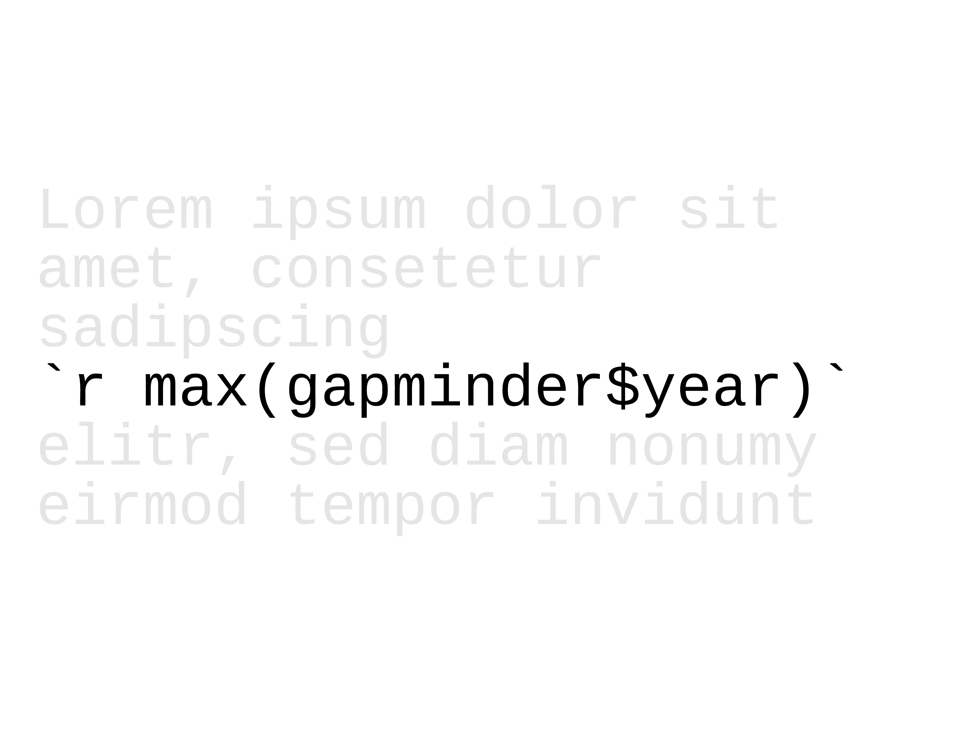
28 / 51
Inline Code
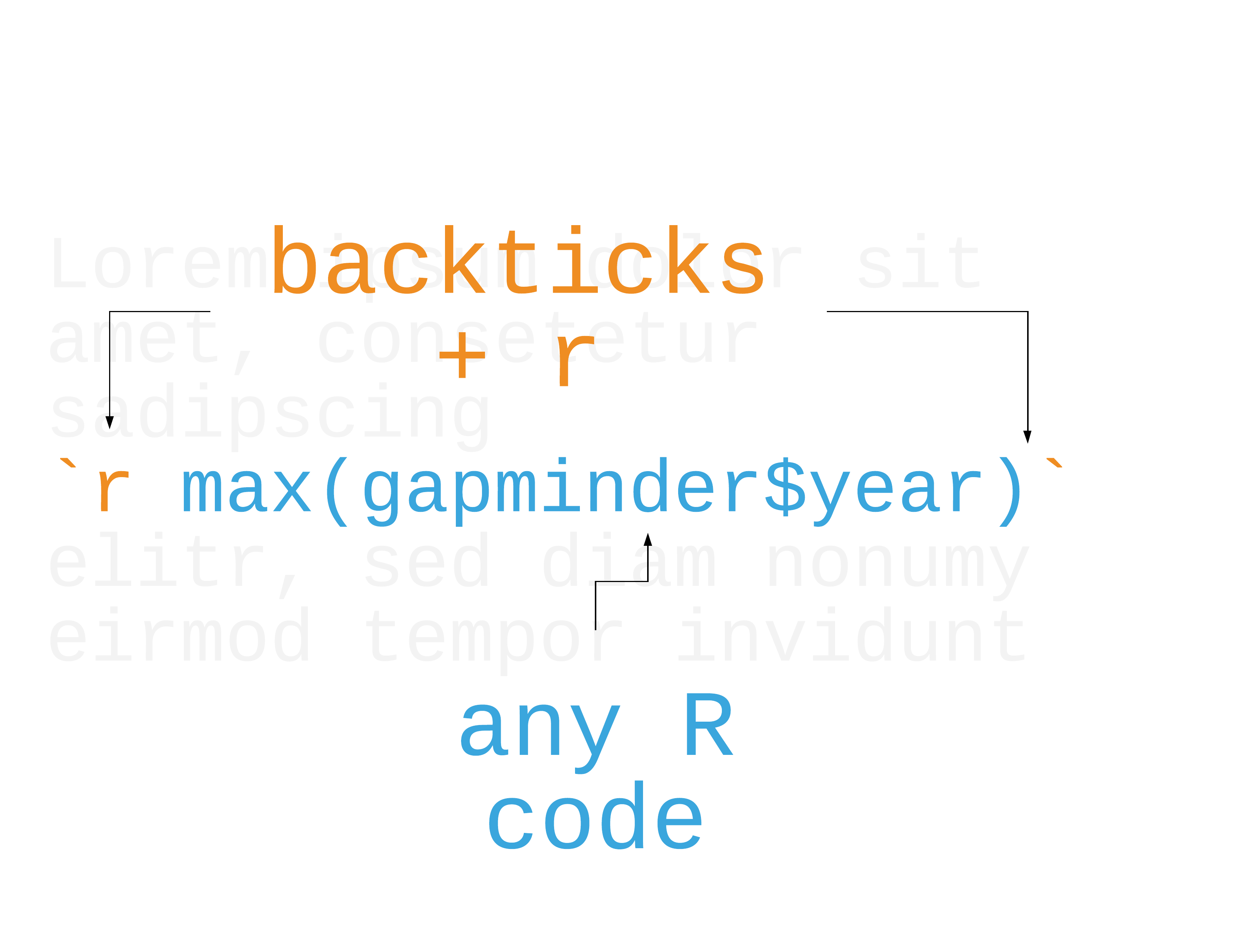
29 / 51
Your turn 6
Remove eval = FALSE so that R Markdown evaluates the code.
Use summarize() and n_distinct() to get the the number of unique years in gapminder and save the results as n_years.
Use inline code to describe the data set in the text below the code chunk and re-knit.
30 / 51
R Markdown
Prose
Code
Metadata = YAML
31 / 51
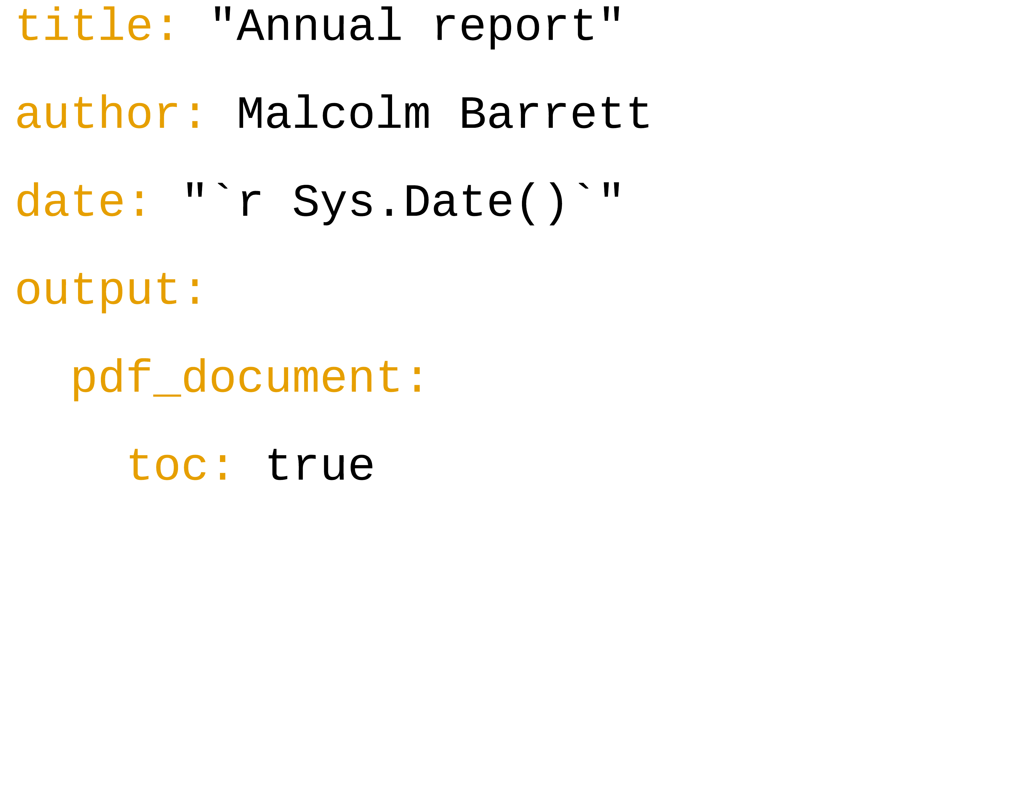
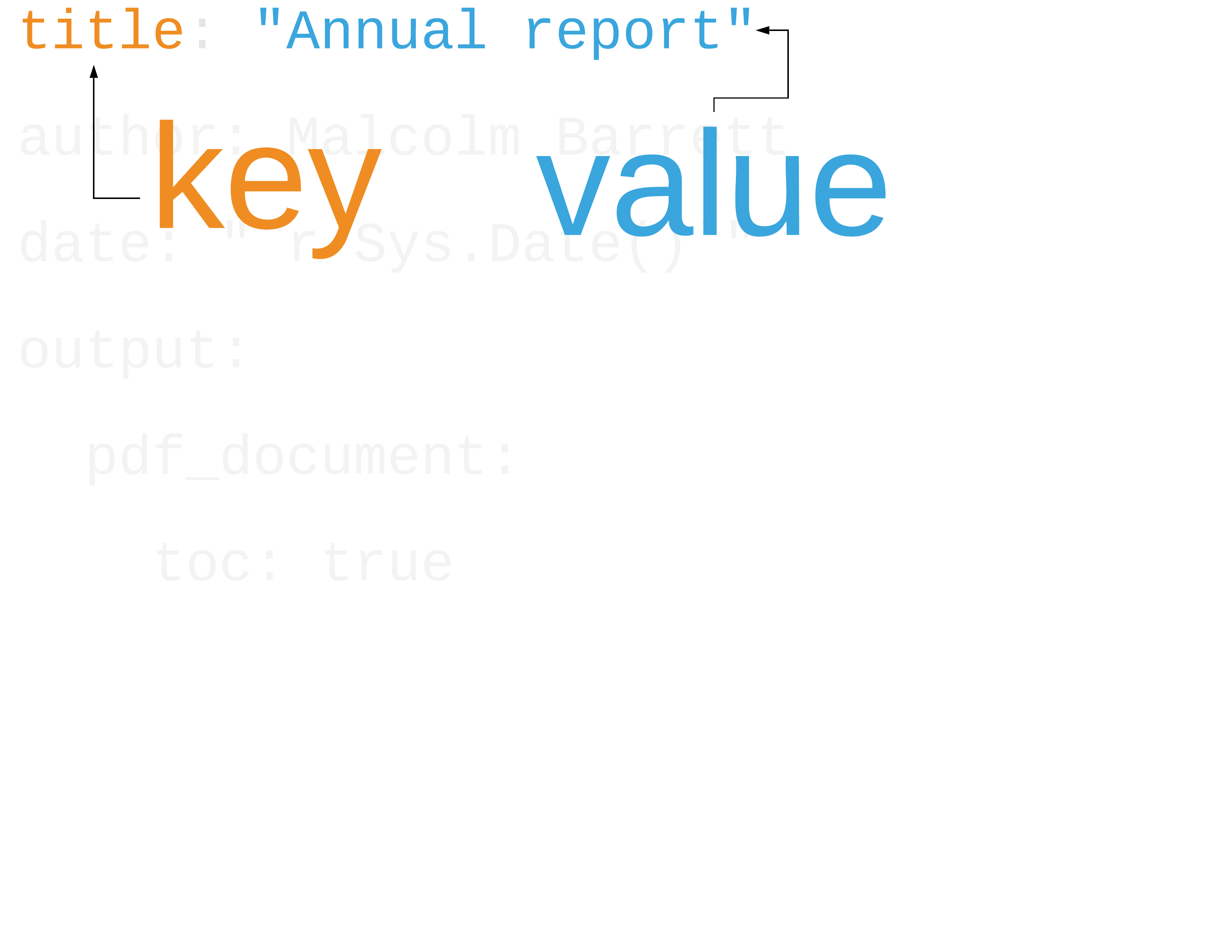
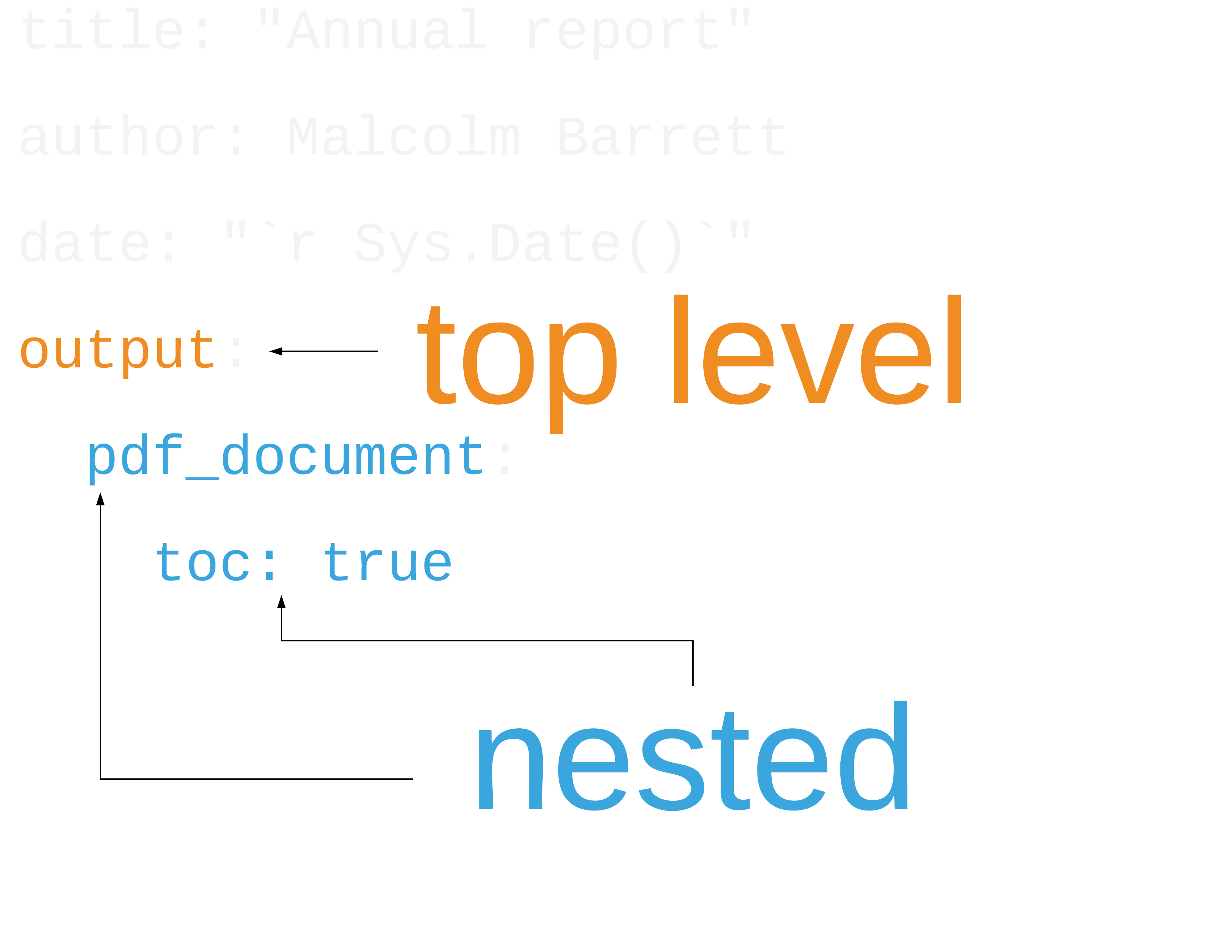
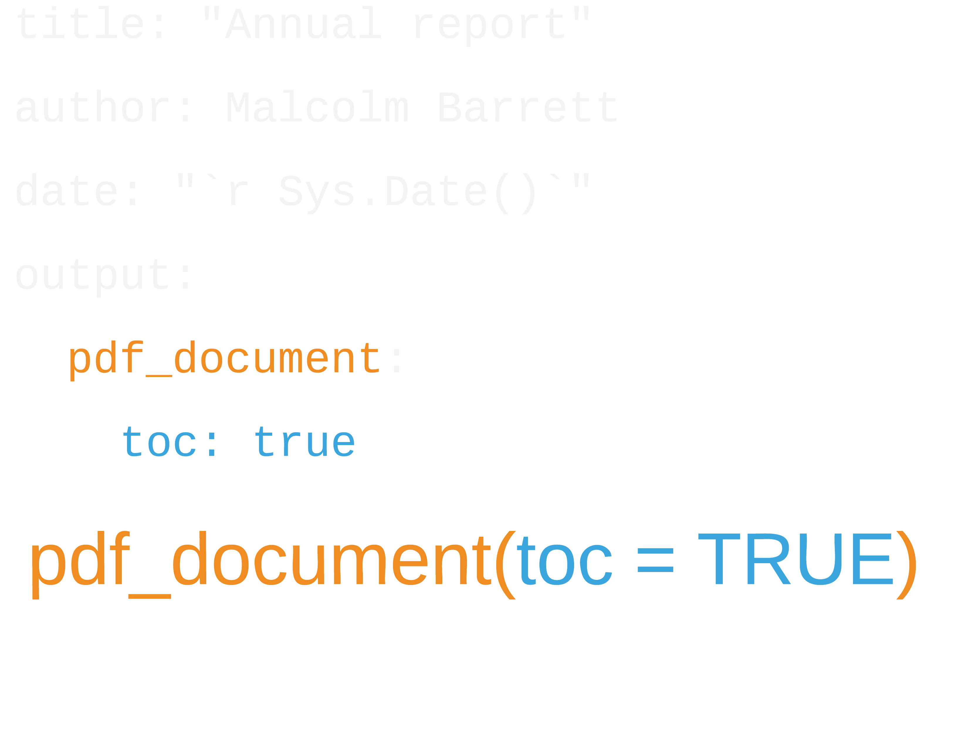
YAML Metadata
---author: Malcolm Barretttitle: Quarterly Reportoutput: html_document: default pdf_document: toc: true---32 / 51
33 / 51
34 / 51
35 / 51
36 / 51
37 / 51
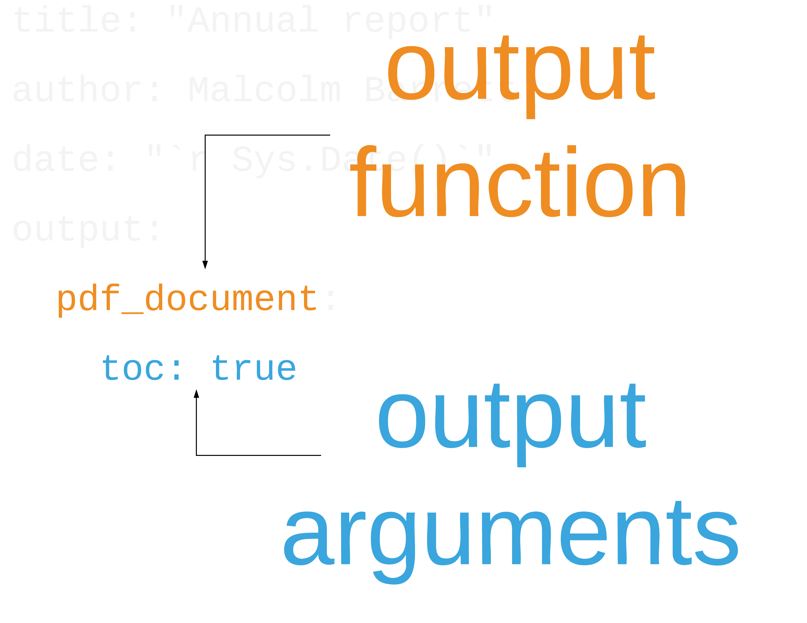
Output formats
| Function | Outputs |
|---|---|
html_document() |
HTML |
pdf_document() |
|
word_document() |
Word .docx |
odt_document() |
.odt |
rtf_document() |
.rtf |
md_document() |
Markdown |
slidy_presentation() |
Slidy Slides (HTML) |
beamer_presentation() |
Beamer Slides (PDF) |
ioslides_presentation() |
ioslides (HTML) |
powerpoint_presentation() |
Powerpoint Slides |
38 / 51
Your turn 7
Set figure chunk options such as dpi, fig.width, and fig.height. Run knitr::opts_chunk$get() in the console to see the defaults.
Change the YAML header above from output: html_document to another output type like pdf_document or word_document.
Add your name to the YAML header using author: Your Name.
39 / 51
ymlthis
check out the ymlthis package for tools and documentation for working with YAML
https://r-lib.github.io/ymlthis/
40 / 51
Parameters
---params: param1: x param2: y data: df---41 / 51
Parameters
---params: param1: x param2: y data: df---params$param1params$param2params$data41 / 51
Your turn 8
Change the params option in the YAML header to use a different continent. Re-knit
gapminder %>% filter(continent == params$continent) %>% ggplot(aes(x = year, y = lifeExp, group = country, color = country)) + geom_line(lwd = 1, show.legend = FALSE) + scale_color_manual(values = country_colors) + theme_minimal(14) + theme(strip.text = element_text(size = rel(1.1))) + ggtitle(paste("Continent:", params$continent))42 / 51
Bibliographies and citations
43 / 51
Bibliographies and citations
Bibliography files: .bib, End Note, others
44 / 51
Bibliographies and citations
Bibliography files: .bib, End Note, others
.bib, End Note, othersCitation styles: .csl
45 / 51
Bibliographies and citations
Bibliography files: .bib, End Note, others
.bib, End Note, othersCitation styles: .csl
.csl[@citation-label]
46 / 51
Including bibliography files in YAML
---bibliography: file.bibcsl: file.csl---47 / 51
Your turn 9
Cite the Causal Inference book in text below in the format [@citation-label]. The label for the citation is hernan_causal_2019
Add the American Journal of Epidemiology CSL to the YAML using csl: aje.csl
48 / 51
Check out the citr package for easy citation insertion and .bib management
49 / 51
Make cool stuff in R Markdown!
bookdown
blogdown
these slides!
50 / 51
Resources
R Markdown: A comprehensive but friendly introduction to R Markdown and friends. Free online.
R for Data Science: A comprehensive but friendly introduction to the tidyverse. Free online.
R Markdown for Scientists: R Markdown for Scientists workshop material.
51 / 51